Oscilloscope

Purpose:  We take a look at the applications of the oscilloscope. With the oscilloscope, we are able to see how the voltage behaves. We are also about to generate various waves and interpret them

The Cathode Ray Tube

We get a look at a cathode ray tube before we begin using the oscilloscopes. A beam is shot from the inside of the tube and it is moved by the electric field. The electric field applies a force on the beam which causes it shift accordingly.

The Oscilloscope And Voltage

The image shows what the reading of voltage is prior to any voltage put it. We can see that it is at the center of the screen, which we say is our zero voltage.

 After, a voltage is put into the oscilloscope and this cause a shift on the vertical line which in this cane indicates our voltage.

Professor Mason goes over the kind of noise that we can get that can be found on top of a DC power supply. The power supply causes a shift of the horizontal line  in the vertical direction. The noise is a variation of the voltage on top of the voltage the power supply says it would put out.

Our board displays a before and after of the power reading from the oscilloscope. We show that the beam is projected with a horizontal velocity and shift upward due to a electric field by the plates located on top and on the bottom.

Setting Up The Function Generator With A Speaker

We connect the function generator to a speaker so and mess with the frequencies to see what kind of noises we hear. We also switch the types of wave outputted by the function generator. We found that these switches effect the sound.

Connecting A Function Generator To An Oscilloscope

We now play with the controls and see how they affect the oscilloscope. Altering the oscilloscope, we can see if voltage is constant or whether it alternates.

Measuring The Change In Voltage

For DC power supplies, we see that we get a constant voltage and the magnitude of this voltage is seen on the oscilloscope when the horizontal line changes position.

Changing The Frequency Signal Of Two Clean Power Supplies

We connect the oscilloscope to two clean power supplies. These supplies create a nice picture when we tinker with the frequency. The shape on the oscilloscope becomes dependent on the two frequencies of the horizontal and vertical axis. 

Summary Of The Oscilloscope

Mystery Box

The image shows some of data collected from the mystery box. Using this data, we interpret what each color does.

Conclusion:  We find that the oscilloscope does a great job in determining the behavior of voltage on a power supply. Using the visual representations on the oscilloscope, we are able to make conclusions on whether a power supply is a DC or AC supply. We are also able to determine whether a DC power supply truly outputs what it says by checking on the oscilloscope for noise.

Charging And Discharging Capacitors

Purpose:  We attempt to find whether capacitors achieve the potential of the power supply instantaneously or if it takes some amount of time for the capacitor to charge. For this, we utilize Logger Pro to see the behavior of potential as a function of time.

Seeing How Capacitors Charge

To begin, we create a circuit with a power supply, a light bulb, and a capacitor. When all are connected, the light bulb shows no light. This is because the circuit is not completed, as there is a break within the capacitor. This break causes no current to flow. But, what we end up seeing, after time has passed, is that when we disconnect the power supply and only connect the capacitor with the light bulb, the bulb lights up and then begins to dim. This means that the capacitor charged while connected to the power supply which makes sense because we have negative charge gathering at one end of the capacitor and positive at the other end, essentially creating a new power supply. But how fast does a capacitor charge?



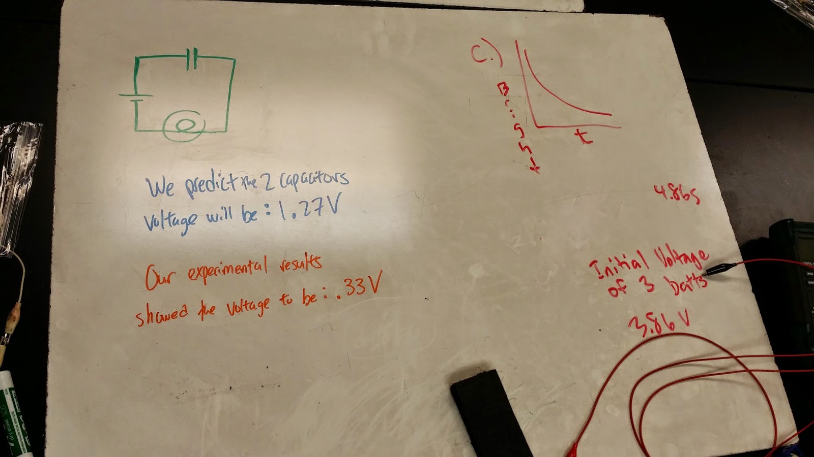
We made predictions for the potential of a capacitor and found that we over estimated the potential.

How Fast Does It Charge

When we graph the potential vs. time of the capacitance, we see that the potential increase exponentially.

Charging Rate Of Capacitors

We hook up a new capacitor to a circuit and connect the capacitor to Logger Pro so that we can examine how the potential changes exponentially.

Rate At Which A Capacitor Charges

As we look at how the capacitor charges, we fit the slope of the line with the closest fit equation which turns out to be some variation of the exponential function. We will later interpret what these values actually mean.

Rate At Which A Capacitor Discharges

We observe how a capacitor discharges and find the it goes at an exponential rate as well. The values of the function will, also, be later interpreted.

Deriving The Potential OF a Capacitor As A Function Of Time

We start off by looking at the general equation for capacitance and make it in terms of the potential. We also know that the potential is dependent on the current and the resistance. When we set these two potential equations equal, we solve for the charge. We know that current can be written as the change in q with respect to time. With a little algebra, we set up two integrals and solve for q. We get a definition for the charge of a capacitor with respect to time. Since the charge is proportional to the potential, we can rewrite this equation by replacing the charges with potentials. This gives us our function for potential with respect to time. This looks very similar to the fit equation found in Logger Pro.

How Long Does It Take For A Potential To Charge

We are given a circuit with a switch and when the switch is closed, the emf charges the capacitor. With the given values, we are able to solve for the time that it takes to charge the capacitor. This just involves using our derived formula and plugging in the values.

We take a look at the same problem, but we look at how long the capacitor takes to reach a charge of an electron. This just requires us to alter the potential equation so that it outputs a charge value.

Conclusion:  We find that capacitors take some time to attain potential as well as charge. We found that this time is dependent on an exponential function. As time passes, the capacitor charges quicker and quicker. The same can be said about discharging. There are slight differences between the equations for charge and discharge but the idea is the this occurs exponentially. When a capacitor is connected to a power supply, it charges, and we can then disconnect the power supply and use the capacitor as a new power supply. The only difference is that the power decreases.

Introduction of Capacitance

Purpose:  We begin to investigate what capacitance is and how it is measured. We also go over some of the methods for finding the total capacitance of a number of capacitors, similar to how we found the equivalent resistance.

Quiz Problem

We begin by going over the quiz. The quiz tested our understand of using Kirchhoff's Laws. We had to create two loops in the circuit and write and equation depicting how the potential drops as we go through the loop. This drop should equal to zero. We, then, utilize the relationship between the currents and these three equations, we are able to find the values for the current at different positions. Once we have the current, we are able to measure potential and this allows us to measure how much power is generated by the circuit.

The Inside Of A Capacitor

Professor Mason takes apart a capacitor and we see that there are two conducting plates separated by some material called a dielectric. What the dielectric does is enhance the capacitance of the capacitor by altering the permittivity.  This is important because the capacitance is proportional to the permittivity. It is also proportional to the area of the plates and inversely proportional to the separation distance.

Finding The Capacitance

We decide to solve for the size of the plates needed in order to have a capacitance of one farad and a separation distance of 1 mm in a vacuum space. We found that we need a square sheet of length 3.55 miles. This seem outrageous. To compensate for the area of the sheet, we can put a dielectric between the sheets. This allows us to use a reasonable size sheet for the same amount of capacitance. This demonstrates the importance of dielectrics in capacitors.

Making A Homemade Capacitor

We begin a hands-on experiment by creating our own capacitors using two sheet of aluminum foil.

We use our lab manual to separate the aluminum. This means that the paper acts as a dielectric. The capacitance is then measured at several different separation distances.

The image shows how we placed the aluminum in the lab manual. WE made sure to stick in deep in the manual to prevent the two foils from touching. If they touch, no capacitance is created. We connect the foil to the multimeter to measure its capacitance.



We then created a chart that signified how the capacitance changes as the distance changes. This created an inverse graph that says, as the separation distance increases, the capacitance approaches zero. As the separation decreases, the capacitance approaches an infinite value. This proves the idea the capacitance is inversely proportional to the separation distance.



Our board shows some of the calculations we had to make in order to make the chart used in the previous picture.

Finding Equivalent Capacitance

Like we did with the resistors, we began to see how the total capacitance is found by orienting the capacitors in parallel and in series. We used the multimeter to find the total capacitance and found that the parallel orientation allows us to just add the capacitors to find the total capacitance. If that is the case, we see that this is opposite of the resistor, so we make a reasonable guess that the series orientation is found using inverse sum. This turns out to be true in the end.

We practice finding the equivalent capacitance of a random oriented layout of capacitance and, again, we must look at piece by piece until everything is simplified and we have one value for all of the capacitors.

An Exploding Capacitor

Professor Mason shows us what happens when we put too much potential in a capacitor. The capacitor ends up blowing up. The reason this occurs is because the space within the plates become conductive by a large electrical field. The electric field rips electrons apart causing the space to become conductive and this causes a short circuit, creating a spark.

Conclusion:  We found that Kirchhoff's Laws prove very useful when evaluating a circuit. We also found that the capacitance is proportional to the area and the permittivity and inversely proportional to the separation distance. The permittivity proves to be very useful because it allows us to make large capacitors without using miles of material. We, also, found the technique for find the equivalent capacitance. This is useful because we can configure capacitors in order to achieve the desired capacitance.

Direct Current Circuits And Resistance

Purpose:  We introduce direct current circuits. We also introduce the idea of resistance, how to orient them and how to measure this orientation.

Circuit 1

Professor Mason begins by demonstrating two kinds of circuits with light bulbs attached. The first is a circuit with a switch at the center wire and the center wire also has a light bulb. The other two light bulbs are are a part of a circuit of one loop when the switch is open and these light bulbs are hooked in series as well as the batteries. The light bulbs in series are on due to the power supplied from the battery. The question is, if we close the switch, will the light at the center turn on. We find that it does not because the potential along the center wire is zero and with no potential, no power to light the bulb.

Circuit 2

In the second circuit, we have the two light bulbs connected in series when the switch is open. The question is, what happens when the switch is closed, introducing a new battery? We find out that the batteries do not change their brightness. This is because the potential drop remains the same, therefore, the power supplied to the bulbs do not change.

Summary Of the Circuits

Our board summarizes what occurred with the light bulbs when we closed the switch, which is no change.

The Introduction Of Resistors

On the top left corner of the board, we make a list of the ways we can configure the light bulbs and the batteries to make the lights dim or bright. We conclude that the brightness is dependent on the voltage and the current. We, then, introduce resistors in series connected to two power supplies in series. We do this to see how the resistance adds up in series. When we measure the resistance using the multimeter, we find the total resistance of the resistors in series is just the sum of the resistors.

Resistance In Parallel

Next, we connect the two resistors in parallel and measure the total resistance. The inverse of the total resistance turns out to be the inverse sum of the resistors.

In the lab manual, we document all of the voltages and current across the two orientations of resistance done previously. We find that the current splits into two smaller current after the first junction and the sum of the two smaller currents is equal to the initial current. If there are no junctions, the current is that same throughout and this current is dependent on the amount of resistance in the circuit.

Reading The Resistance Of Resistors

On the left hand side of the board, there are a bunch of resistors. These resistor have color markings on them so that a person can determine the resistance. The way to do this is to find the initial color and final color. The final color will determine the tolerance of the resistance while the color next to it is called the multiplier. This multiplier just multiplies the number received by the initial colors. The initial colors indicate single digits that determine the magnitude of the resistance and this is multiplied by the multiplier if it is larger by 10n times the digits found.

Finding The Equivalent Resistance

To get the hang of finding the equivalent resistance, we start off by finding equivalent resistance of a simple orientation of resistors.

In this image, the resistors are oriented more randomly. The key here is to find equivalent resistance of parts of the circuit, until it looks like a simple parallel or series orientation. For example, we start by looking at the top left parallel wires. We know how to add parallel resistors but we can only do it if the is one representation of resistance on each wire. We get this single representation by first finding the single representation of the two resistors in series, then, we find the equivalent resistance of the parallel wires. We keep doing this, little by little, until we had a single resistance that represents all of the resistors.

Conclusion:  We found that the key to a light bulbs brightness depends on the potential difference as well as the current, which is the power. This is proved by the first two circuits, especially the first. Our group believed the the middle bulb would turn on because flipping on the switch would introduce current. But the potential difference turned out to be zero and this causes no power to be supplied. We found out how to read the resistance of a typical resistor. These values are determined using colored strips. We, also, found a way for getting the equivalent resistance of any orientation. This is important because it allows us to get the desired resistance using a multitude of fix values of resistors.

Electric Potential

Purpose:  We, further, go into the concept of electric potential by going over some examples that are different than just two point charges. We, also, go into some hands-on activities for electric potential.

Potential Of A Charged Ring

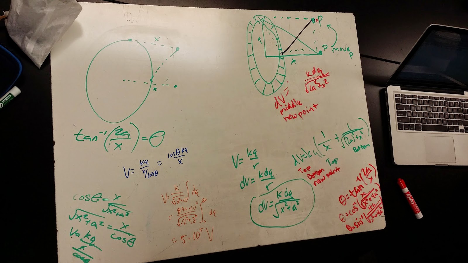
To begin our first potential problem, he had a ring with some charge on it. We then knew the variable dimensions of the ring and the potential point we are trying to find. The first point is in the center of the ring at some x distance away. We, then, start with the standard equation for potential, but this only applies to point charges. We alter the equation by saying the change in our potential is proportional to the change in q. After, we integrate to find the potential.

Potential Of A Charged Ring At A Different Location

Next, we use the same ring to find the potential at a different location. The twist here is that the location is positioned where it is difficult to take advantage of symmetry because the point is positioned at the top corner of the ring at some distance away. The key here is getting the proper distance that the point is from the ring. Using geometric representations, we are able to find that it is an x distance away from the ring and if a is the radius of the ring, we can say that the potential changes as the a distance increase and decreases.It increases and decreases because as we are taking infinitesimally small segments of dq, we integrate around the ring. This changes the a value. We can express this in terms of the change in the angle and solve for the potential.

Finding Potential Using E-Field

We work with the first problem of a charged ring and find the potential at a point x away from the ring centered in the middle of the ring. This time, we solve for the electric field the charged ring produces and use the definition for potential to solve for the potential of the ring at that distance. By definition, the potential difference is equal to the negative integral of the dot product of the electric field and the distance from infinity to the distance. When we solve for the potential this way, we get the same conclusion we saw before.

Using Excel To Find Potential

We continue with a different problem that is similar to the ring. This time, we have a wire of the length and solve for its potential and distance above the wire at the center of the wire using an excel spreadsheet. We decided to break the ring into 20 segments. We, then, solve for the potential at a segment using the center of the segment as the point charge. Once we have the potential of one segment, we multiply by the number of segments. This gives us nearly the same numerical value for potential of the ring.

We continue to solve for the same wire problem but we approach it differently. Instead, we look at the change in the radial distance and the potential it has throughout this change. This is very similar to the integral method. Once we have the potentials at every distance, we add up all of the potentials and in the end, we and up with the same answer we received from the previous excel sheet.

Potential By Integration

We can find the potential of a wire at any distance above it using the integral method. We determine the the y component does not change but the x does. We the write of an equation for the potential that expresses the change in the x direction. If we know where the point we are looking for is positioned with respect to the wire, we can easily solve for the potential using integration with the correct integration bounds.

Finding Potentials Along A Dipole

We start a hands-on experiment for finding the potential. We use a piece of conducting paper and this paper is nailed down to some insulating material. The nails are given an opposite charge and this creates a dipole along the conductive paper. Using the red and black pins, we are able to measure the potential at any point with respect to one of the charges.

This is how we set up the experiment. We hooked up our nails to some power supply. We, then used the multimeter to measure the potential at any point on the conductive paper.

This image includes a summary of our findings for the experiment. After finding the potentials along the x-axis, we were able to find the potential difference as well as the work required to move a charge from one location to the other. Finding the work just requires us to find the potential difference and then multiplying by the value of the charge we are trying to move. This is consistent, as energy is equal to the potential times the charge.

We found that as the radial distance approaches zero, we get infinite potential and as the radial distance approaches infinity, we get zero potential.

Conclusion:  We experimented with various ways to find potential from a distribution of charge. These methods include excel arithmetic and integration. Depending on the charged figure, it may be easier to use an excel sheet to find potential. We, also, received a hands-on view of potential when we determined the potential at various points of a dipole. We conclude that potential is zero infinitely far away and infinite at the source.