Torque And Flux

Purpose:  We examine how the electric field effects two charges that create a dipole. We, then, use VPython to view get a 3 dimensional representation of the electric field of a dipole. At the end, we will encounter flux.

Electric Projectile

When we look at two sheets of metal, we see that in the example given, the electric field moves in one direction. When looking at a particle that is charged and contains a velocity pointing parallel to the planes, we see that the motion it exhibits is that of a projectile.

Moment of a Dipole

Using a visual representation of a dipole in the are of the electric field, we say that a torque is create between. The dipole moment is then used to find the potential energy, as we took the integral of the moment with respect to theta, the rotational distance. We find that the dipole moment is the cross product of the separation distance by the force. We also find that the potential energy is the dot product of the moment of the dipole by the electric field.

Prediction vs. VPython

The program initially set up is displayed by the red arrows pointing to the right. The green arrows demonstrate the prediction of the electric field line of a dipole. When comparing to the VPython visual representation, we saw that our prediction was not far off. We predicted using a general idea of the sum of the electric fields.

After we finished a 2 dimensional representation of the electric field on a dipole, we went a little further and created a 3 dimensional representation of a dipole electric field.

The drawing above shows how the electric field on a dipole looks like.

Flux

We show the different ways flux is dawn, in opposite directions of the same object. We see that flux is used to determine the amount of electric field lines that pass through a surface. 

Flux occurs in only 2 sides of a cube when the cube is oriented along the x,y, and z axis and when the electric field points along only one of the axis. The other surfaces are facing parallel to the electric field, cause no field lines to cross the surface. The net flux is still zero, as the flux in cancels the flux out. 

Conclusion:  We found that the electric field cause a charge particle to accelerate in a linear direction and even graphed a 3 dimensional representation of the electric field lines of a dipole. We can see that its a mess as many arrows shoot off into many directions. We, then, take a look at the flux. The flux is given by the electric field lines that pass through a surface, or the integral of E dot with dA.

The Electric Field

Purpose: In this lab, we will take a look at the concept of electrical fields. We will also use VPython to show a 3 dimensional representation of an electric field.

Definition of The Electric Field

We start by interpreting the electric field in the same manner as gravity, but we changed some of the words to fit the description of the electric field.

We  know that the electric field is the electrical force divided by the charge the force is exerted on. Therefore, we can make a comparison, where our charge is like mass and the electric field is like the acceleration in Newton's second law.

The Sum of The Electric Fields

On our board, we show a visual representation of all the point charges having an electric fied that converges at a test charge. Like in problems involving gravity, we can use superposition to find the net electric field on a test charge.

On the board, an example of finding the net electric field is displayed. The test charge is to the right of the two charges and on charge is positive while the other is negative.

The next example for solving for the net electric field involves a test charge in between the two opposite charges, a distance above the origin. Using vector analysis, we were able to successfully find the net electric field. The y component cancels while the x component adds in the negative direction.

Using Excel For Computations

On excel, we were able to quickly solve for the net electric field of a rod when we put a test charge next to the end of the rod. the test charge is a distance from the end of the rod.

By inputting the givens in a electric field problem, we were able to solve for the electric field quickly for a problem with changing x and r values. Normally, a problem like this would take much longer by hand, but on excel, we are able to put the necessary equations to solve for the net electric field. This problem was very similar to the previous excel problem except the test charge was in the center of the rod, above the rod. We also had to account for the thickness of the rod, as we were looking at center points in a cylinder.

We take a look at the problem done in the first excel picture, but calculated it without excel. We integrated to find the sum of the electric field. The tricky part was getting the correct limits of integration, as we had to remember that the test charge was not directly next to the end of the rod but a distance away from it.

Electric Field on VPython

On VPython, we set up an axis with a particle of positive charge. We then show the behavior of the electric field using arrows. This was done using Professor Mason's template.

Conclusion:  We see that the electric field of a charge shoots outward or inward radially. We also see that, when finding the net electric field on a test charge, the rule of superposition applys, making calculations fairly simple. We can make comparisons between Newton's second law and the force equation for electric force. We, also, learn that using excel makes calculations faster and easier if done properly.

3 Dimensional Objects in VPython

Purpose:  To getting a better understanding of vectors in three dimensions, we learn a little bit of computer programming. This lab represents the work done in learning some of the basic programming skills in VPython.

Getting The Hang Of Things

As soon as I watched the video about how to create 3 dimensional objects in space, I began to create 3 spheres in different positions. I didn't realize that the spheres would be in contact with each other.

I, then, reduced the size of the spheres to get a little separation. I could have also changed the position but for the sake of getting used to manipulating the spheres, I decided to see if I could change their size on the first try.

Next, I created an arrow attached to a sphere and pointed it in the negative x direction, to see how it looked.

Once I got the hang of manipulating the arrows, I began to orient them in the same manner as in the tutorial.

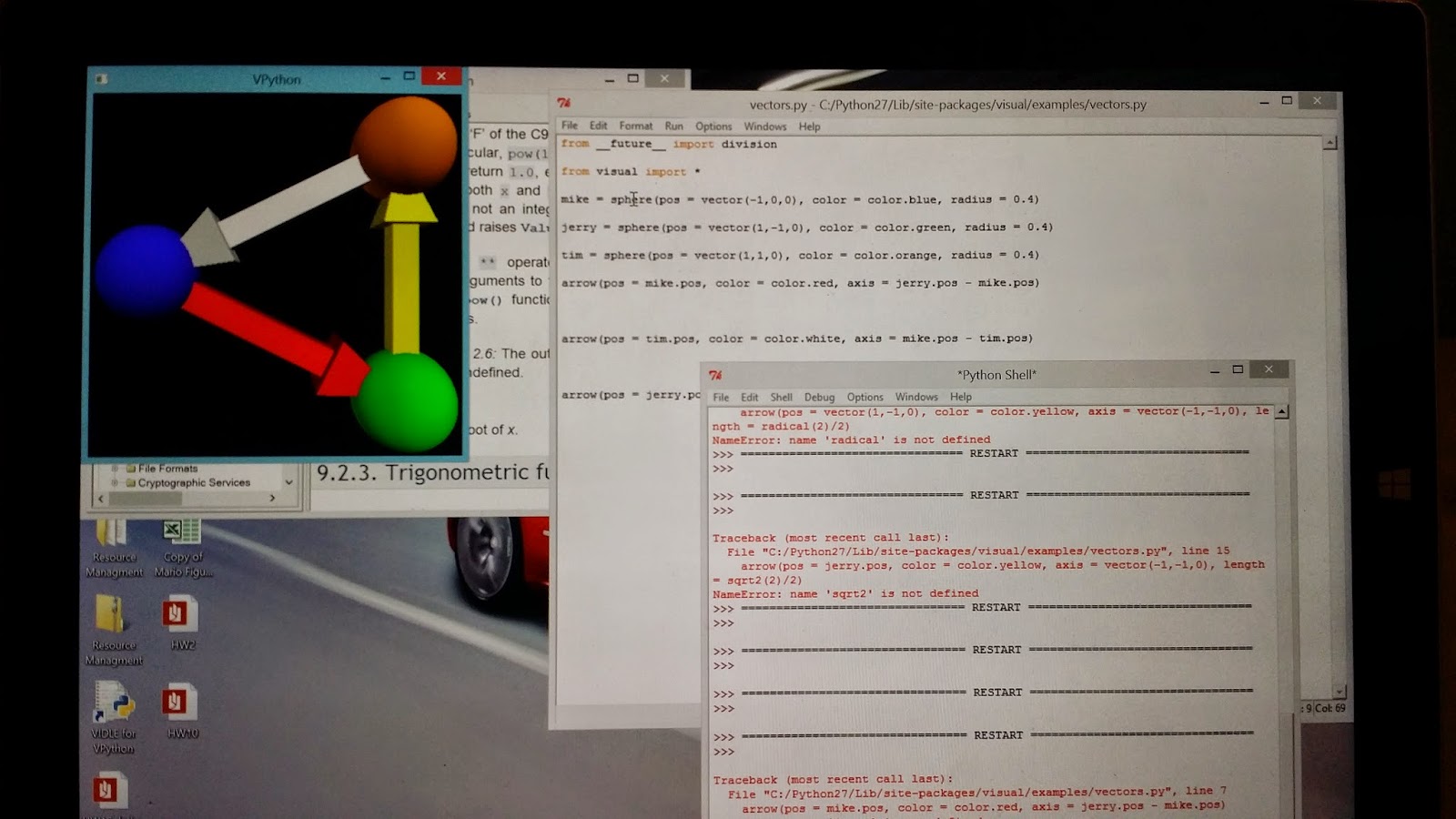
Once the arrows were positioned correctly, I changed the colors of the spheres and the arrows. The large amounts of red font shows my failure to produce a color that VPython could recognize.

After I finished changing the colors, I played around with the pound sign that allows me to ignore code. The pound sign highlights everything that proceeds it on the same line and does not use it for the program.

Then next step was to orient the arrows so that they may touch the neighboring spheres in a counter-clockwise fashion. It was a bit tricking, as I stumbled into some coding problems. I did not remember that when I give something a name, I can only recall it if the name was stated at the beginning. I fixed this by changing the structure of the lines and the program worked.

This picture shows how the arrows change when I push a sphere upward by double its distance. The arrows, definitely, change in length.

This shows how the print option works

This shows that I am using the newer version of VPython and can write the print option in either of the two ways shown.

Conclusion:  VPython shows that it can be picky in the way the directions are organized but it is a great way to view a 3 dimensional object.

Charge

Purpose:  In this experiment, we observe how charges behave when they are near each other. We also prove that there are two kinds of charge, one positive and one negative.

A Charged Balloon

We start off by rubbing a balloon. This balloon was rubbed against Professor Mason's hair and stuck to the glass that the balloon was next to. This is because the balloon lost some electrons during the rubbing process and became positively charged. When held next to the glass, the electrons in the glass gathered toward the positively charged balloon, causing an attraction.

Charged Tape

We take another look at charge when we charge tape by quickly separating tape that is taped on each other. The two pieces of tape stick to each other because on tape becomes positively charge by losing electron to the other tape. This make the other tape negatively charged. This shows that positive and negative charges attract.

We then ask ourselves, " how can we show that there are actually two charges in play?" Well, we do the same thing shown in the previous picture but with a second set of tape as well, giving us four pieces of tape. when we charge all of these pieces of tape in the same manner, some of the tapes repel, and some attract, showing that there are pieces of tape that gain the same charge and that there are two kinds of charge.

As part of the observation of the two tapes, we had to come up with explanations for why the tape behaved the way it did. This is what we came up with.

Charge Using Newtons Laws

In this problem, we went oldschool as we applied Newtons Laws to find the electrical force done on the charged ball.

Using the force we found using Newton's Laws, we found a relationship between Force and R. We can see that the force falls at one over R squared.

Same Charges Don't Attract

We take a closer look at the behavior of two charges by mapping out their positions. The red dots track the motion a man holding a charged ball on a stick and the green dots track the motion of a charged ball that hangs on a string.

Using the same equation for electrical force derived using Newton's Laws, we were able to get Logger Pro to calculate the force on the ball. We, then, graphed a force versus distance graph and, again, it shows that the force is inversely proportional to the separation distance of the two same charge objects.

Here is some of the numerical data obtained.



This picture contains a detailed analysis of our fit equation for the force of the two charged balls on Logger Pro. The fit equation was raised to the power of negative 2 and this is consistent with the equation for force of an electric charge.

This picture contains some more analysis. Number 4 shows where some uncertainty lies in the experiment.

We take a look at two opposite charge balls and these charges have the same charge in magnitude. We see that the force of the charges follow Newton's third law.

Franklin Motor

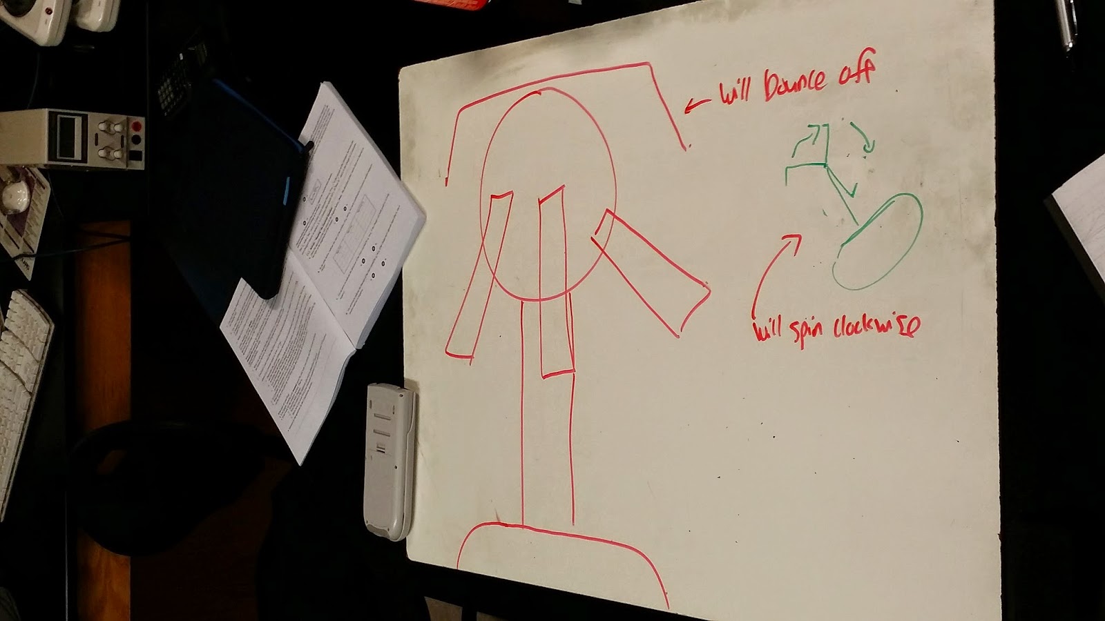
We start off by see how the paper would react to vandegraff generator. Most of us were able to guess that the paper would move in the way shown in the picture.



The paper from the previous picture shows us that it is resisting gravitational pull, so, we calculated the ratio between the force of gravity and the force of electric charge. Electric charge is roughly ten raised to the power of 40, which shows that it is much strong than gravity.

When we set up the Franklin motor, we see that the top spins clockwise. The charge is dispersed to the ends of the three metals that spin.

Our picture shows our prediction of the direction of the rotation as well as the reaction with the paper. Both of our predictions were true.

Conclusion:  Step by step, we prove that there are two charges at work when we talk about electrical charge. This was proven using tape. We, then, used Newton's Laws to see the force of electric charge and plugged this formula in Logger Pro to find the behavior of force versus separation distance. The graph showed some inverse proportionality, which we fitted, and we found the force was inversely proportional to separation distance squared. We talked about the application of Newton's third law and went into different examples of charging objects. The behavior proved to be a little predictable.

Hot and Cold Reservoirs and Entropy

Purpose:  We examine the importance of entropy and how it is relevant in our standard PV diagrams. We also look into diagrams involving entropy and solving these diagrams in a similar manner as our PV diagrams.

The Fan

We examine a sterling engine which runs on temperature difference. The fan spins, showing work is being done.

We decide to switch the temperature reservoirs and, like the experiment with the disk, the fan spins in the opposite direction, again, showing what happens when we switch the reservoirs.

Temperature vs. Entropy Diagram

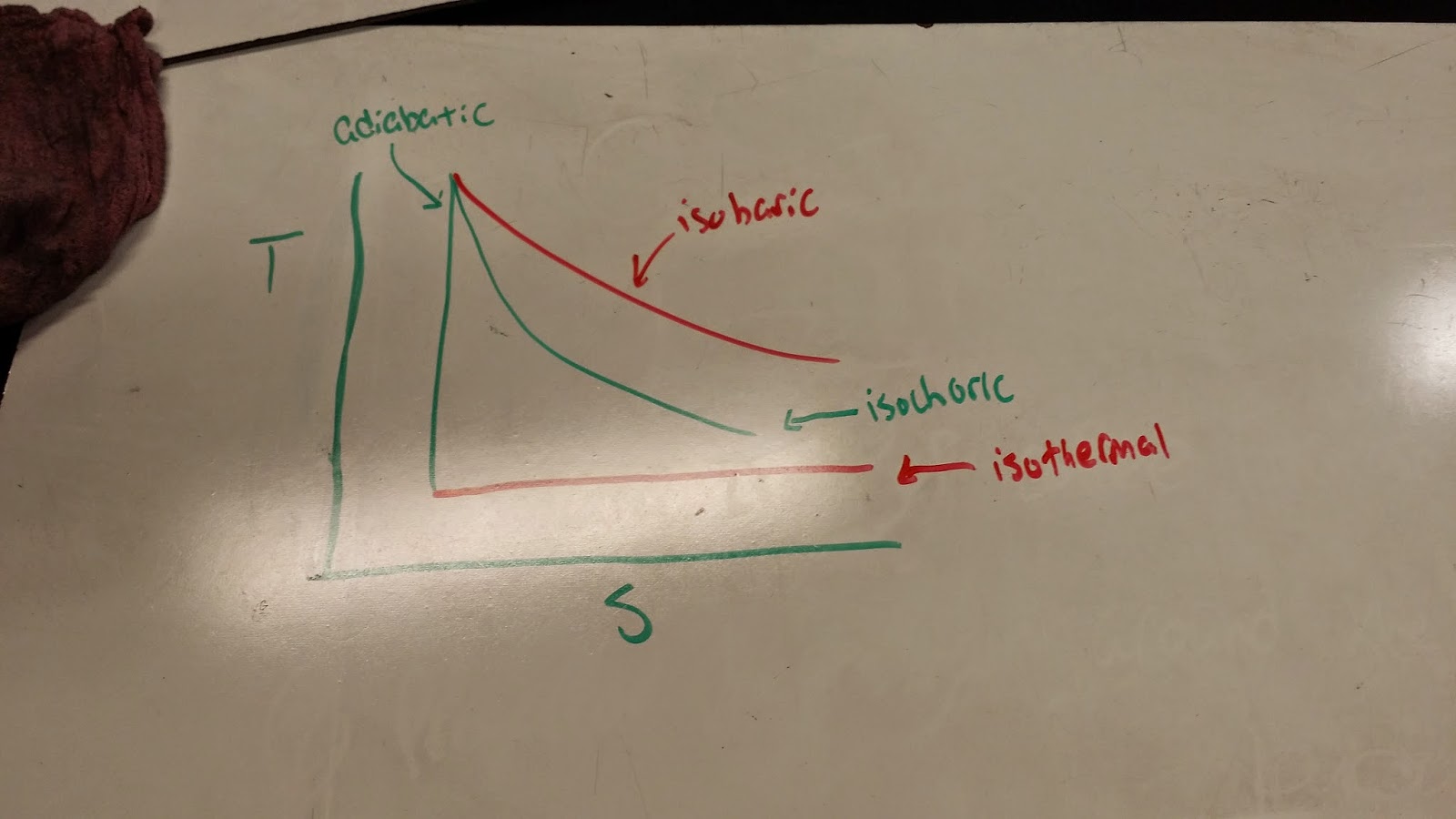
We look at our first temperature versus entropy diagram and see that the diagram looks awfully similar to some standard pressure versus volume diagrams. In a temperature versus entropy diagram, the adiabatic assumes the behavior of the isochoric process and the isothermal process assumes the behavior of the isobaric process and the isochoric and isobaric assume the adiabatic and isothermal behavior, respectively. This makes sense as temperature is constant in isothermal processes and there is no change in heat in an adiabatic processs, causing no change in entropy.

We examine the maximum possible efficiency the sterling engine could produce by calculating the efficiency of a carnot engine. Again, this efficiency is not attainable, but a good theoretical value to make sure are efficiency is reasonable.

The Coefficient of Performance

We use the coefficient of performance to find the heat required to warm a home with the temperature outside being very cold and the temperature inside being room temperature.

How Effective Is It?

We take a look at effectiveness of an engine. Our effectiveness is given by the net work divided by the work of a reversible processes. This, then, translates into the actual efficiency divided by the efficiency of a reversible process.

Zero Change in Entropy

We look at an example where two objects sit next to each other until thermal equilibrium is reached. Both objects have different temperature and the change in entropy is zero. We, then, solve for final temperature.

After we have found our final temperature, we then find the work done. We know that heat is equal to mass time the specific heat times the change in temperature. We also know that work is hot heat minus the cold heat.

Using only the given temperatures, we solve for the coefficient of performance. This allowed us to find the hot Heat.

Finally, we use what we know about heat flow to find the time it takes to freeze something. 

Bubbles Experiment

We see that when Professor Mason blows air through a tube, creating a bubble, The bubble immediately falls to the ground because the bubble is more dense than the air.

We see in the second part of the experiment that the bubble rises up. This is because there is no air inside the bubble, as it was replace with a gas less dense than air.

We use a lighter to lit the methane bubble on fire and as we lit it, the flame went upward. This makes sense since we light the bubble from the bottom and it travels in the same direction as the methane gas.

Conclusion:  We ventured into entropy as we viewed how a temperature versus entropy diagram looks with the same four processes found in our standard PV diagrams. The difference between the two is that the area in a temperature versus entropy diagram shows us the heat transferred to the gas, not the total work done. We also found the coefficient of performance, a value that similar to the efficiency and a value of effectiveness. Using these, we ventured into practical applications. We finished off by looking at a bubble. One bubble with more density and one bubble with less density. Then, we lit the bubble with less density in flames to observe the direction the flame travels.